Molecular Simulations: The Fun Way to Predict Binding Affinity

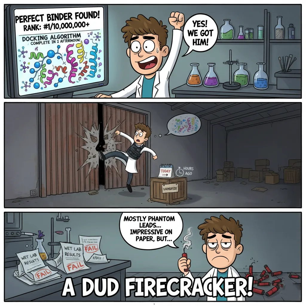
Picture a thriller where the hero tracks down the villain using perfect surveillance footage, kicks down the warehouse door, and finds nothing. The target vanished hours ago. This is exactly what happened when our docking algorithm ranked millions of "perfect" binders in an afternoon. The wet lab results? Most were phantom leads, impressive on paper but in reality, most of them were a dud firecracker.
Just like static surveillance can't capture real movement, molecular docking gives us beautiful snapshots that miss the dynamic reality of molecular life. This disconnect between computational prediction and experimental truth is the central challenge of structure-based drug discovery. Docking, as I explained in my previous article on molecular docking, is an efficient starting point. But it’s still a snapshot: proteins are treated as mostly rigid, water is simplified, and entropy is largely ignored.
Beyond Static Snapshots
Proteins are not frozen sculptures; they flex and shift in solution, revealing hidden pockets or collapsing apparent ones. Docking can’t capture this motion or the entropy cost of locking a flexible ligand into place, which often explains why “perfect” binders fail experimentally. Molecular dynamics (MD) simulations step in here, running proteins and ligands in motion over nanoseconds to microseconds, letting us see if a pose is truly stable. Coupled with methods like free energy perturbation (FEP), MD brings us closer to realistic binding affinities than docking ever could.
These limitations of docking are not just theoretical nitpicks. Large benchmarking efforts, like the D3R Grand Challenges [1], repeatedly show how docking struggles in practice. Even when a ligand’s pose looks right with less than 2 Å deviation from the crystal structure, the scoring functions often misjudge the actual binding strength. Flexible receptors, solvent effects, and entropy penalties are simplified or skipped altogether, so docking scores drift away from experimental affinities. The result: plausible poses but poor predictions.
We are on a mission to make molecular and structural biology related experiments easier than ever. Whether you are doing research on protein design, drug design or want to run and organize your experiments, LiteFold helps to manage that with ease. Try out, it's free.
Simulating Life in Silico
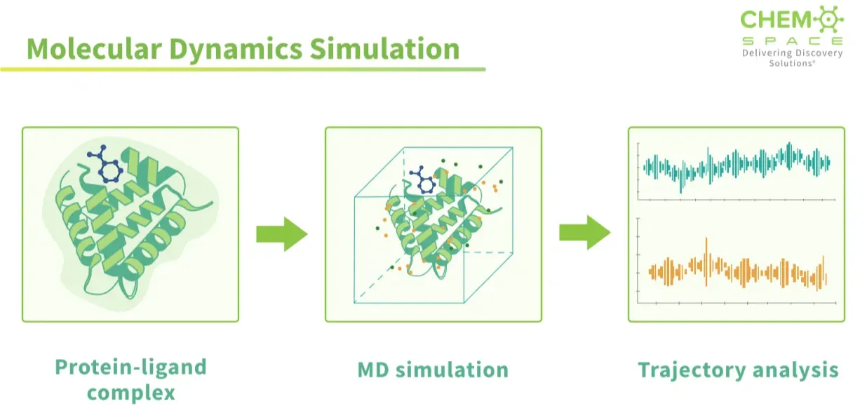
Docking is a snapshot; molecular dynamics is the movie. In MD, the computer doesn’t just line up shapes and call it a match. It actually solves Newton’s equations of motion for every atom, protein, ligand, and even the surrounding water. The result is a frame-by-frame movie of how the system behaves in time. Side chains wiggle, water molecules drift in and out, and the binding pocket, sometimes opening wider, sometimes shut immediately. Instead of a rigid lock-and-key guess, MD shows the interaction as it really is: alive, flexible, and constantly shifting. This is powerful for two reasons:
- Refinement: It tells you if a docking pose is stable or falls apart once the protein undergoes conformational change.
- Thermodynamics: From the trajectory, you can estimate binding free energy , essentially, how favorable it is for the ligand to stay bound versus floating away.
These calculations are extremely tedious often needing long simulations (hundreds of nanoseconds, sometimes microseconds) to see meaningful motions, especially for flexible targets thus using a lot of computational recourses.
Force Fields and why it matters so much
If molecular dynamics is a movie, then the force field is the script. Atoms don’t know physics on their own, computers need a set of rules that say how strongly bonds stretch, how angles bend, how charges attract and how van der Waals forces push and pull. To simply put, a force field is set of equations and parameters that translate Newton’s laws into numbers the simulation can run with.
Different MD software packages implement these rules in slightly different ways. Some focus on biomolecular accuracy, others on speed, GPU performance, or flexibility for custom setups. Table 1 (below): Some of the most widely used MD engines handle force fields and related features:
| MD Engine | Best For | Force Field Specialties | Performance Considerations | Accessibility |
|---|---|---|---|---|
| AMBER | Proteins, nucleic acids, small molecules | AMBER (ff14SB, ff19SB) for proteins; GAFF/GAFF2 for drug-like molecules | Good CPU scaling, improving GPU support | Free for academics, paid for commercial use |
| CHARMM | Membrane proteins, lipid bilayers, carbohydrates | CHARMM36 for proteins and lipids; CGenFF for drug-like molecules | Extensive tools for setup and analysis | Academic source code access, commercial licenses required |
| GROMACS | Large biomolecular systems, membrane proteins | Compatible with most force fields Optimized for AMBER and CHARMM | Excellent CPU scaling, highly efficient code | Open source, free for all uses |
| OpenMM | Method development, custom protocols | Compatible with standard force fields and Excellent for custom force fields | Best GPU performance, flexible programming model | Open source, Python API makes it accessible |
| OPLS | Drug discovery, organic molecules | OPLS-AA and OPLS-2005/OPLS3e for proteins and drug-like molecules | Optimized for Schrödinger software suite | Commercial license through Schrödinger |
The role of Enhanced Sampling and Binding Free Energies
MD is great for short clips, but it is painfully slow. Most simulations runs are in microseconds, while the real biology happens on the millisecond-to-second scale. It’s like trying to watch a 2-hour film by capturing a few seconds of footage, you miss the big plot twists.
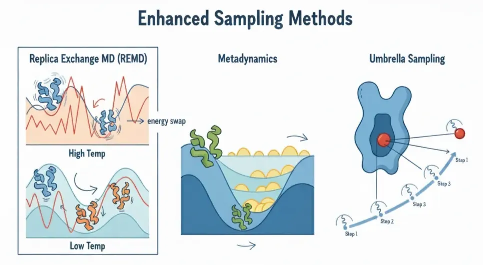
That’s where Enhanced Sampling Methods come in: they tweak the rules of the movie so we can fast-forward through the boring parts and jump to the rare, high-impact scenes. Just like there’s no single shortcut to skipping boring scenes in a movie, there isn’t one trick to speeding up MD. Some popular approaches include:
- Replica Exchange MD (REMD):In normal MD, the system is stuck because at room temperature it doesn't have the energy to hop over barriers. REMD solves this by running clones of the same system at different temperatures. High-temp replicas shake harder, cross barriers more easily, and then occasionally trade places with the low-temp replicas.Result: the cold replicas get access to high-energy states they'd never reach on their own.
- Metadynamics:Proteins love to sit in the same comfy valley. Metadynamics continuously adds small "energy hills" (Gaussians) to discourage the system from revisiting the same states, flattening the landscape so it explores new conformations.
- Umbrella Sampling:Some processes, like pulling a ligand out of a protein pocket, are so energetically steep that doing it in one go doesn't work, the ligand just falls back in. Umbrella sampling breaks the journey into small, manageable steps, each stabilized with a gentle restraint (a spring).
- Other tricks (ABF, Funnel MD, etc.):These are more specialized, but they all share the same idea: add just enough bias to help the system cross barriers, then carefully remove the bias in analysis to get the true physics back.
Once we’ve explored these states and confirmed that the ligand actually stays bound, the next big question is: “How strong is that binding?”
This is where binding free energy (ΔG_bind) comes in. It’s the number that tells us, quantitatively, how tightly a ligand grips its protein, directly related to the experimental dissociation constant (Kd).
Computing it is hard because you need to capture both enthalpy (the energy of interactions) and entropy (the freedom molecules lose when they stick together). Over the years, computational chemists have built a toolbox of methods that trade accuracy for speed.
- Docking scores are fast, great for triaging huge libraries, but not real free energies.
- Molecular Mechanics Poisson-Boltzmann Surface Area (MM-PBSA) takes MD snapshots, calculates energies for bound vs. unbound states, and adds implicit solvation. It’s cheap and sometimes gets trends right, but absolute errors can be brutal.
- Linear Interaction Energy and Extended LIE (LIE/ELIE) estimate binding free energy by focusing on the main interactions between a ligand and its protein, electrostatics and van der Waals forces. Combining this energies and a few coefficients (learned from experimental binding data), reasonably increases prediction.
- Free Energy Perturbation (FEP ) is the heavyweight champion. It literally “alchemically” morphs one ligand into another inside the protein pocket across a series of simulations. Done carefully, it reaches near-experimental accuracy. The catch: it eats a lot of compute and requires expertise.
Table 2 (below): Overview of Computational Methods for Estimating Binding Free Energy.
| Method | Principle | Strengths | Weaknesses |
|---|---|---|---|
| Docking Score | Empirical / force-field scoring of poses | Very fast, screens millions | Not a true free energy; ignores entropy |
| MM-PBSA | Energy + solvation (PB/GB) from MD snapshots | Cheap, widely used | High errors (>6 kcal/mol), sensitive to setup |
| LIE / ELIE | Empirical scaling of interaction energies | Faster than FEP, better than MM-PBSA | Needs training, poor transferability |
| FEP | Alchemical transformation of ligands | Near-experimental accuracy | Heavy compute, expert setup |
The Limits of Classical Force Fields
For decades, simulations have leaned on classical force fields like AMBER, CHARMM, and OPLS. They’ve been workhorses, aiding in countless discoveries and drug design projects. But they’re not flawless. But simplicity comes at a cost.
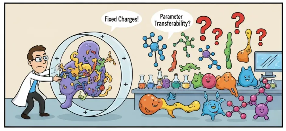
The biggest issue? Fixed charges. Real molecules aren’t static; their electron clouds shift, polarize, and sometimes even transfer charge between atoms. Classical force fields freeze those charges in place, which makes them less accurate for charged or highly polar systems.
Another problem is parameter transferability. A force field calibrated for one class of molecules may break down for another, forcing researchers into tedious re-parameterization before they can even hit “run.”
Neural Network Force Fields: The New Frontier
This is where machine learning steps in. Neural network force fields don’t start with a fixed equation, they learn the energy landscape directly from high-level quantum mechanical (QM) data, calculations which capture how electrons really behave. Because they learn directly from QM, these models can “feel” things classical models can’t. For example:
- Polarization: In reality, the electron cloud around an atom distorts when another charge comes nearby. Classical force fields freeze charges in place, but neural nets can respond dynamically.
- Charge transfer: Sometimes electrons actually shift from one molecule to another (common in binding pockets). Classical models can’t handle that, but neural nets can.
- Many-body effects: Instead of treating each interaction pair by pair (like atom A pulling on atom B), neural nets can capture the collective influence of multiple atoms acting at once.
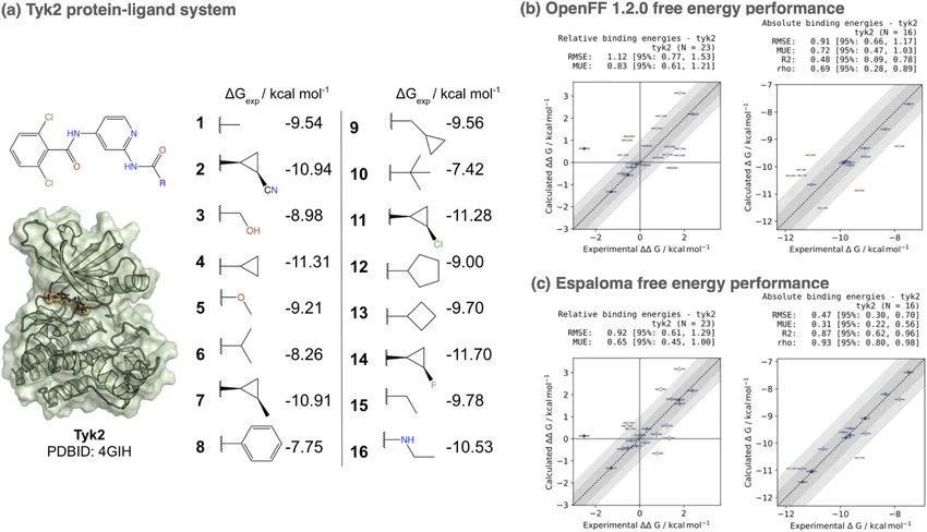
The difference isn’t just theoretical. In one benchmark, the neural network force field Espaloma beat a widely used classical force field (OpenFF 1.2.0) for the Tyk2 kinase system, cutting prediction error from 1.10 kcal/mol down to 0.73 kcal/mol. In drug discovery, where fractions of a kcal/mol can reorder your entire hit list, that’s a big deal [3].
How an MD Simulation Actually Run?
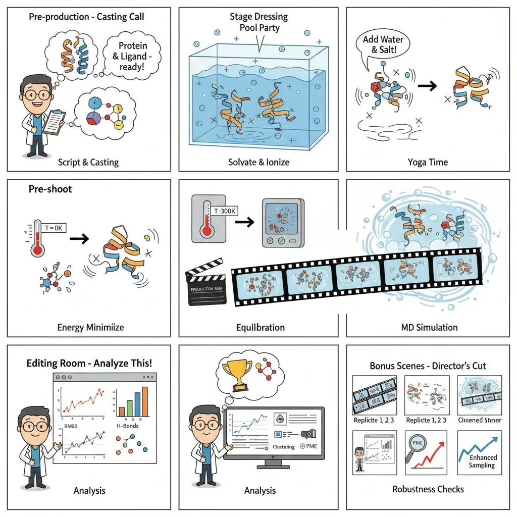
Picture MD as building a movie studio. You set the stage with physical laws, then capture the dynamic dance of atoms. While traditional MD requires arcane command-line knowledge, modern platforms like Litefold.ai simplify this complexity into intuitive interfaces.
- System Setup; The Script & Cast: We begin by preparing the protein and ligand, fixing missing atoms, assigning charges, and choosing a force field. A bad setup here is like miscasting the lead actor, the whole show falls apart.
- Environment Creation; Setting the Stage: Molecules don’t live in a vacuum. We place them in a water box, add ions, and mimic physiological salt levels. This ensures the interactions unfold in something resembling real biology.
- Energy Minimization; Safety Check: Before rolling the cameras, we need to relax any tense spots in our molecular system. This step removes any unrealistic high-energy positions that could cause the simulation to crash. Otherwise, the simulation could “explode” from bad starting positions.
- Equilibration; The Rehearsal: Now we gently warm the system to body temperature (300K), holding the main structure steady while water and side chains find their natural rhythm. This step ensures everything is stable before the real run.
- Production Run; The Filming: This is the actual simulation. The restraints come off, the system runs freely, and we record atomic motion over nanoseconds to microseconds. These snapshots become our molecular movie.
- Analysis: The Editing Room: Once the movie’s shot, we dig into the frames: tracking RMSD, hydrogen bonds, conformational changes, or calculating binding free energies. This is where raw motion turns into scientific insight.
- Validation & Enhancement; Quality Control: Finally, we check consistency by running repeats, ensuring the results are statistically solid. If needed, we apply enhanced sampling to capture rare but important events.
Where MD Still Falls Short
MD gives us incredible atomic detail, yet there are walls it can’t break. There are several reasons for that. For example:
1. The Timescale Problem: Simulations run for nanoseconds to microseconds, but biology moves on milliseconds to seconds. It’s like trying to understand a symphony by sampling a few microseconds of each note. Enhanced sampling helps, but we’re still orders of magnitude away from the true pace of life.
2. The Accuracy Ceiling: Even the best free energy methods top out at ~0.5–1.0 kcal/mol accuracy. Sounds tiny, but in binding affinity that’s a 3–5x error. In drug discovery, where the difference between nanomolar and micromolar binding can decide success or failure, that margin reshuffles your hit list.
3. The Transferability Gap: No force field or neural net works everywhere. Something tuned for soluble proteins may flop on membrane proteins; trained on kinases, it may stumble on GPCRs. There’s no universal recipe, every new target demands painful re-validation.
4. The Sampling Myth: Even with enhanced methods, you never know if you’ve really seen everything. A hidden allosteric pocket might only open at the 10-millisecond timescale, and your microsecond run won’t catch it. Missing those rare states can mean missing the mechanism of resistance or selectivity.
5. The Computational Reality Check: Yes, AI force fields and FEP can approach experimental accuracy. But they eat compute for breakfast and demand expertise. Academic labs and small biotech are stuck between costly “rigorous” methods and cheap-but-dodgy approximations like MM-PBSA.
6. The Validation Bottleneck: The real choke point isn’t silicon, it’s biology. You can run a thousand MD jobs in a week, but testing ten compounds in the lab takes months.
The bottom line? It’s brilliant for understanding mechanisms, generating hypotheses, and prioritizing experiments. Just don’t confuse computational confidence with biological truth. The wet lab still has the final word.
Conclusion
Molecular dynamics is not just an add-on to docking. It is the bridge between static prediction and biological reality. By letting proteins and ligands “breathe” in silico, MD helps separate true binders from false positives, refines docking poses, and allows a first look at the thermodynamic cost of binding. It does not eliminate the need for experiments, but it dramatically narrows the search space and gives wet-lab teams higher-quality hypotheses to test.
The future of MD lies at the intersection of physics and machine learning. Neural network force fields, GPU acceleration, and better enhanced-sampling protocols are already pushing simulations toward biological timescales and near-experimental accuracy. Combined with smart triaging (docking, FEP, AI-driven pose scoring), MD will remain one of the most valuable tools for turning computational predictions into actionable leads. The goal is not just to simulate reality but to guide it, prioritizing the right molecules, reducing wasted syntheses, and accelerating the path from idea to drug.
References
[1] D3R Grand Challenge Overview – Community-wide evaluation of computational drug design methods.
[2] Chemspace – Molecular Dynamics Simulations: Concepts and Applications
We are on a mission to make molecular and structural biology related experiments easier than ever. Whether you are doing research on protein design, drug design or want to run and organize your experiments, LiteFold helps to manage that with ease. Try out, it's free.